A job of hours now done in seconds!

A guy has to process an excel file everyday where there is a column having some kind of reference numbers as shown in column ‘A’ below:

As per requirement of his work, he needs to remove the special characters from these numbers and make them like the values shown in column ‘B’. He used to edit each one manually to remove the special characters. There are hundreds of reference numbers. So, it took hours to accomplish this.

One fine morning he asked me to suggest a shortcut way to do that.

I wrote a very simple program and now it’s a one-click job.

You can also install it in your computer. Follow the following steps to install :

Firstly Download the program named ‘Extractum’

Open MS Excel.

Click the ‘Office Button’ at the top left corner

Click ‘Excel Options’

 Click ‘Add-ins’ in the left

At the bottom of the Add-ins list, select ‘Excel Add-ins’ beside ‘Manage’ (if not selected by default)

Click ‘Go…’ button

A list of available add-ins will appear

Click ‘Browse…..’

Now show the location of ‘ExtractNum’

Click ‘Ok’

Now it is installed in your computer. You can use it as shown in the image above (cell B2). Now if there are thousands of cell in a column containing such data, it is matter of few seconds to remove the special characters.

Do you need any such help?

Please feel free to comment here or contact ExcelAccessHelp@gmail.com.

Very simple yet Very useful!

Say, you have many numbers in an excel sheet.

You want to divide all the numbers with say 100.

How to do that?

You can do this in several ways. However, the simplest way is as follows:

1.       Write 100 in a cell in the sheet

2.       Copy it

3.       Select the data you want to divide

4.       Click right button on the selected data

5.       Choose ‘Paste Special’

6.       In the ‘Paste Special’ dialogbox, check the ‘Divide’ radio button under operation group

7.       Click ‘Ok’

Now all the data you selected will be divided by 100.

Want to let me know your problem?

Please comment or send email to ExcelAccessHelp@gmail.com

Solution to a common problem of Chart in EXCEL.

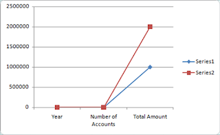
Normally we make chart in Excel by selecting the data and then choosing a chart type under the insert menu. However, if there is huge difference among the data, the chart may look bizarre. Solution to such a problem is discussed below:

Say, your data is

You want to make a chart like this

If you select your data and from insert menu select a line chart type, your chart will looks like this

Solution:

Right click the chart.
In the pop-up menu Choose ‘Select Data’.
The following dialogbox appears:

In the dialogbox, click ‘Sereies 1’, then click edit. The following dialogbox appears:

Click in the ‘Sereies name’ box, then click on ‘Number of Accounts ’.

Click the arrow next to the ‘Sereies values’ box, then select values in the ‘Number of Accounts’ column like this:

Click OK.

Click on ‘Series 2’. , then click 'Edit'.

Click in the ‘Sereies name’ box, then click on ‘Total Amount ’.

Click the arrow next to the ‘Sereies values’ box, then select values in the ‘Total Amount’ column.

Click OK.

Now click on ’Edit’ under ‘Horizontal (Category) Axis Labels’. Select the data in ‘Year’ column (i.e., 2016, 2017).

Click OK.

Now the chart looks like:

Click on the line representing ‘Series 1’.

Select Chart Tools>Format Format Selection:

Following dialogbox will appear.

Click ‘Series Options (if not selected).
Check ‘Secondary Axis’ radio button.
Click close.

Now your chart will look like:

If needed, choose display options under ‘Layout’ tab in the ‘Chart Tools’.

Continue visiting my blog for useful tips and solutions.
Please contact ExcelAccessHelp@gmail.com for consultancy on EXCEL and ACCESS.